Modeling Non-linear Least Squares
Introduction
Ceres solver consists of two distinct parts. A modeling API which provides a rich set of tools to construct an optimization problem one term at a time and a solver API that controls the minimization algorithm. This chapter is devoted to the task of modeling optimization problems using Ceres. Solving Non-linear Least Squares discusses the various ways in which an optimization problem can be solved using Ceres.
Ceres solves robustified bounds constrained non-linear least squares problems of the form:
In Ceres parlance, the expression
\(\rho_i\left(\left\|f_i\left(x_{i_1},...,x_{i_k}\right)\right\|^2\right)\)
is known as a residual block, where \(f_i(\cdot)\) is a
CostFunction that depends on the parameter blocks
\(\left\{x_{i_1},... , x_{i_k}\right\}\).
In most optimization problems small groups of scalars occur together. For example the three components of a translation vector and the four components of the quaternion that define the pose of a camera. We refer to such a group of scalars as a parameter block. Of course a parameter block can be just a single scalar too.
\(\rho_i\) is a LossFunction. A LossFunction is
a scalar valued function that is used to reduce the influence of
outliers on the solution of non-linear least squares problems.
\(l_j\) and \(u_j\) are lower and upper bounds on the parameter block \(x_j\).
As a special case, when \(\rho_i(x) = x\), i.e., the identity function, and \(l_j = -\infty\) and \(u_j = \infty\) we get the usual unconstrained non-linear least squares problem.
CostFunction
For each term in the objective function, a CostFunction is
responsible for computing a vector of residuals and Jacobian
matrices. Concretely, consider a function
\(f\left(x_{1},...,x_{k}\right)\) that depends on parameter blocks
\(\left[x_{1}, ... , x_{k}\right]\).
Then, given \(\left[x_{1}, ... , x_{k}\right]\),
CostFunction is responsible for computing the vector
\(f\left(x_{1},...,x_{k}\right)\) and the Jacobian matrices
-
class CostFunction
class CostFunction {
 public:
  virtual bool Evaluate(double const* const* parameters,
                        double* residuals,
                        double** jacobians) const = 0;
  const std::vector<int32>& parameter_block_sizes();
  int num_residuals() const;

 protected:
  std::vector<int32>* mutable_parameter_block_sizes();
  void set_num_residuals(int num_residuals);
};
The signature of the CostFunction (number and sizes of input
parameter blocks and number of outputs) is stored in
CostFunction::parameter_block_sizes_ and
CostFunction::num_residuals_ respectively. User code
inheriting from this class is expected to set these two members with
the corresponding accessors. This information will be verified by the
Problem when added with Problem::AddResidualBlock().
-
bool CostFunction::Evaluate(double const *const *parameters, double *residuals, double **jacobians) const
Compute the residual vector and the Jacobian matrices.
parametersis an array of arrays of sizeCostFunction::parameter_block_sizes_.size()andparameters[i]is an array of sizeparameter_block_sizes_[i]that contains the \(i^{\text{th}}\) parameter block that theCostFunctiondepends on.parametersis nevernullptr.residualsis an array of sizenum_residuals_.residualsis nevernullptr.jacobiansis an array of arrays of sizeCostFunction::parameter_block_sizes_.size().If
jacobiansisnullptr, the user is only expected to compute the residuals.jacobians[i]is a row-major array of sizenum_residuals x parameter_block_sizes_[i].If
jacobians[i]is notnullptr, the user is required to compute the Jacobian of the residual vector with respect toparameters[i]and store it in this array, i.e.jacobians[i][r * parameter_block_sizes_[i] + c]= \(\frac{\displaystyle \partial \text{residual}[r]}{\displaystyle \partial \text{parameters}[i][c]}\)If
jacobians[i]isnullptr, then this computation can be skipped. This is the case when the corresponding parameter block is marked constant.The return value indicates whether the computation of the residuals and/or jacobians was successful or not. This can be used to communicate numerical failures in Jacobian computations for instance.
SizedCostFunction
-
class SizedCostFunction
If the size of the parameter blocks and the size of the residual vector is known at compile time (this is the common case),
SizeCostFunctioncan be used where these values can be specified as template parameters and the user only needs to implementCostFunction::Evaluate().template<int kNumResiduals, int... Ns> class SizedCostFunction : public CostFunction { public: virtual bool Evaluate(double const* const* parameters, double* residuals, double** jacobians) const = 0; };
AutoDiffCostFunction
-
class AutoDiffCostFunction
Defining a
CostFunctionor aSizedCostFunctioncan be a tedious and error prone especially when computing derivatives. To this end Ceres provides automatic differentiation.template <typename CostFunctor, int kNumResiduals, // Number of residuals, or ceres::DYNAMIC. int... Ns> // Size of each parameter block class AutoDiffCostFunction : public SizedCostFunction<kNumResiduals, Ns> { public: // Instantiate CostFunctor using the supplied arguments. template<class ...Args> explicit AutoDiffCostFunction(Args&& ...args); explicit AutoDiffCostFunction(std::unique_ptr<CostFunctor> functor); explicit AutoDiffCostFunction(CostFunctor* functor, ownership = TAKE_OWNERSHIP); // Ignore the template parameter kNumResiduals and use // num_residuals instead. AutoDiffCostFunction(CostFunctor* functor, int num_residuals, ownership = TAKE_OWNERSHIP); AutoDiffCostFunction(std::unique_ptr<CostFunctor> functor, int num_residuals); };
To get an auto differentiated cost function, you must define a class with a templated
operator()(a functor) that computes the cost function in terms of the template parameterT. The autodiff framework substitutes appropriateJetobjects forTin order to compute the derivative when necessary, but this is hidden, and you should write the function as ifTwere a scalar type (e.g. a double-precision floating point number).The function must write the computed value in the last argument (the only non-
constone) and return true to indicate success.For example, consider a scalar error \(e = k - x^\top y\), where both \(x\) and \(y\) are two-dimensional vector parameters and \(k\) is a constant. The form of this error, which is the difference between a constant and an expression, is a common pattern in least squares problems. For example, the value \(x^\top y\) might be the model expectation for a series of measurements, where there is an instance of the cost function for each measurement \(k\).
The actual cost added to the total problem is \(e^2\), or \((k - x^\top y)^2\); however, the squaring is implicitly done by the optimization framework.
To write an auto-differentiable cost function for the above model, first define the object
class MyScalarCostFunctor {
  MyScalarCostFunctor(double k): k_(k) {}

  template <typename T>
  bool operator()(const T* const x , const T* const y, T* e) const {
    e[0] = k_ - x[0] * y[0] - x[1] * y[1];
    return true;
  }

 private:
  double k_;
};
Note that in the declaration of
operator()the input parametersxandycome first, and are passed as const pointers to arrays ofT. If there were three input parameters, then the third input parameter would come aftery. The output is always the last parameter, and is also a pointer to an array. In the example above,eis a scalar, so onlye[0]is set.Then given this class definition, the auto differentiated cost function for it can be constructed as follows.
auto* cost_function
    = new AutoDiffCostFunction<MyScalarCostFunctor, 1, 2, 2>(1.0);
                                                    ^  ^  ^
                                                    |  |  |
                        Dimension of residual ------+  |  |
                        Dimension of x ----------------+  |
                        Dimension of y -------------------+
In this example, there is usually an instance for each measurement of
k.In the instantiation above, the template parameters following
MyScalarCostFunction,<1, 2, 2>describe the functor as computing a 1-dimensional output from two arguments, both 2-dimensional.By default
AutoDiffCostFunctionwill take ownership of the cost functor pointer passed to it, ie. will call delete on the cost functor when theAutoDiffCostFunctionitself is deleted. However, this may be undesirable in certain cases, therefore it is also possible to specifyDO_NOT_TAKE_OWNERSHIPas a second argument in the constructor, while passing a pointer to a cost functor which does not need to be deleted by the AutoDiffCostFunction. For example:MyScalarCostFunctor functor(1.0) auto* cost_function = new AutoDiffCostFunction<MyScalarCostFunctor, 1, 2, 2>( &functor, DO_NOT_TAKE_OWNERSHIP);
AutoDiffCostFunctionalso supports cost functions with a runtime-determined number of residuals. For example:auto functor = std::make_unique<CostFunctorWithDynamicNumResiduals>(1.0); auto* cost_function = new AutoDiffCostFunction<CostFunctorWithDynamicNumResiduals, DYNAMIC, 2, 2>( std::move(functor), ^ ^ ^ runtime_number_of_residuals); <----+ | | | | | | | | | | | Actual number of residuals ------+ | | | Indicate dynamic number of residuals --------+ | | Dimension of x ------------------------------------+ | Dimension of y ---------------------------------------+
Warning
A common beginner’s error when first using
AutoDiffCostFunctionis to get the sizing wrong. In particular, there is a tendency to set the template parameters to (dimension of residual, number of parameters) instead of passing a dimension parameter for every parameter block. In the example above, that would be<MyScalarCostFunction, 1, 2>, which is missing the 2 as the last template argument.
DynamicAutoDiffCostFunction
-
class DynamicAutoDiffCostFunction
AutoDiffCostFunctionrequires that the number of parameter blocks and their sizes be known at compile time. In a number of applications, this is not enough e.g., Bezier curve fitting, Neural Network training etc.template <typename CostFunctor, int Stride = 4> class DynamicAutoDiffCostFunction : public CostFunction { };
In such cases
DynamicAutoDiffCostFunctioncan be used. LikeAutoDiffCostFunctionthe user must define a templated functor, but the signature of the functor differs slightly. The expected interface for the cost functors is:struct MyCostFunctor { template<typename T> bool operator()(T const* const* parameters, T* residuals) const { } }
Since the sizing of the parameters is done at runtime, you must also specify the sizes after creating the dynamic autodiff cost function. For example:
auto* cost_function = new DynamicAutoDiffCostFunction<MyCostFunctor, 4>();
cost_function->AddParameterBlock(5);
cost_function->AddParameterBlock(10);
cost_function->SetNumResiduals(21);
Under the hood, the implementation evaluates the cost function multiple times, computing a small set of the derivatives (four by default, controlled by the
Stridetemplate parameter) with each pass. There is a performance tradeoff with the size of the passes; Smaller sizes are more cache efficient but result in larger number of passes, and larger stride lengths can destroy cache-locality while reducing the number of passes over the cost function. The optimal value depends on the number and sizes of the various parameter blocks.As a rule of thumb, try using
AutoDiffCostFunctionbefore you useDynamicAutoDiffCostFunction.
NumericDiffCostFunction
-
class NumericDiffCostFunction
In some cases, its not possible to define a templated cost functor, for example when the evaluation of the residual involves a call to a library function that you do not have control over. In such a situation, numerical differentiation can be used.
Note
TODO(sameeragarwal): Add documentation for the constructor and for NumericDiffOptions. Update DynamicNumericDiffOptions in a similar manner.
template <typename CostFunctor,
          NumericDiffMethodType method = CENTRAL,
          int kNumResiduals,  // Number of residuals, or ceres::DYNAMIC.
          int... Ns>          // Size of each parameter block.
class NumericDiffCostFunction : public
SizedCostFunction<kNumResiduals, Ns> {
};
To get a numerically differentiated
CostFunction, you must define a class with aoperator()(a functor) that computes the residuals. The functor must write the computed value in the last argument (the only non-constone) and returntrueto indicate success. Please seeCostFunctionfor details on how the return value may be used to impose simple constraints on the parameter block. e.g., an object of the formstruct ScalarFunctor { public: bool operator()(const double* const x1, const double* const x2, double* residuals) const; }
For example, consider a scalar error \(e = k - x'y\), where both \(x\) and \(y\) are two-dimensional column vector parameters, the prime sign indicates transposition, and \(k\) is a constant. The form of this error, which is the difference between a constant and an expression, is a common pattern in least squares problems. For example, the value \(x'y\) might be the model expectation for a series of measurements, where there is an instance of the cost function for each measurement \(k\).
To write an numerically-differentiable class:CostFunction for the above model, first define the object
class MyScalarCostFunctor {
  MyScalarCostFunctor(double k): k_(k) {}

  bool operator()(const double* const x,
                  const double* const y,
                  double* residuals) const {
    residuals[0] = k_ - x[0] * y[0] + x[1] * y[1];
    return true;
  }

 private:
  double k_;
};
Note that in the declaration of
operator()the input parametersxandycome first, and are passed as const pointers to arrays ofdoubles. If there were three input parameters, then the third input parameter would come aftery. The output is always the last parameter, and is also a pointer to an array. In the example above, the residual is a scalar, so onlyresiduals[0]is set.Then given this class definition, the numerically differentiated
CostFunctionwith central differences used for computing the derivative can be constructed as follows.auto* cost_function = new NumericDiffCostFunction<MyScalarCostFunctor, CENTRAL, 1, 2, 2>(1.0) ^ ^ ^ ^ | | | | Finite Differencing Scheme -+ | | | Dimension of residual ------------+ | | Dimension of x ----------------------+ | Dimension of y -------------------------+
In this example, there is usually an instance for each measurement of k.
In the instantiation above, the template parameters following
MyScalarCostFunctor,1, 2, 2, describe the functor as computing a 1-dimensional output from two arguments, both 2-dimensional.NumericDiffCostFunction also supports cost functions with a runtime-determined number of residuals. For example:
auto functor = std::make_unique<CostFunctorWithDynamicNumResiduals>(1.0);
auto* cost_function
    = new NumericDiffCostFunction<CostFunctorWithDynamicNumResiduals,
                                           CENTRAL, DYNAMIC, 2, 2>(
        std::move(functor),                            ^     ^  ^
        runtime_number_of_residuals); <----+           |     |  |
                                           |           |     |  |
                                           |           |     |  |
          Actual number of residuals ------+           |     |  |
          Indicate dynamic number of residuals --------+     |  |
          Dimension of x ------------------------------------+  |
          Dimension of y ---------------------------------------+
There are three available numeric differentiation schemes in ceres-solver:
The
FORWARDdifference method, which approximates \(f'(x)\) by computing \(\frac{f(x+h)-f(x)}{h}\), computes the cost function one additional time at \(x+h\). It is the fastest but least accurate method.The
CENTRALdifference method is more accurate at the cost of twice as many function evaluations than forward difference, estimating \(f'(x)\) by computing \(\frac{f(x+h)-f(x-h)}{2h}\).The
RIDDERSdifference method[Ridders]_ is an adaptive scheme that estimates derivatives by performing multiple central differences at varying scales. Specifically, the algorithm starts at a certain \(h\) and as the derivative is estimated, this step size decreases. To conserve function evaluations and estimate the derivative error, the method performs Richardson extrapolations between the tested step sizes. The algorithm exhibits considerably higher accuracy, but does so by additional evaluations of the cost function.Consider using
CENTRALdifferences to begin with. Based on the results, either try forward difference to improve performance or Ridders’ method to improve accuracy.Warning
A common beginner’s error when first using
NumericDiffCostFunctionis to get the sizing wrong. In particular, there is a tendency to set the template parameters to (dimension of residual, number of parameters) instead of passing a dimension parameter for every parameter. In the example above, that would be<MyScalarCostFunctor, 1, 2>, which is missing the last2argument. Please be careful when setting the size parameters.
Numeric Differentiation & Manifolds
If your cost function depends on a parameter block that must lie on a manifold and the functor cannot be evaluated for values of that parameter block not on the manifold then you may have problems numerically differentiating such functors.
This is because numeric differentiation in Ceres is performed by perturbing the individual coordinates of the parameter blocks that a cost functor depends on. This perturbation assumes that the parameter block lives on a Euclidean Manifold rather than the actual manifold associated with the parameter block. As a result some of the perturbed points may not lie on the manifold anymore.
For example consider a four dimensional parameter block that is interpreted as a unit Quaternion. Perturbing the coordinates of this parameter block will violate the unit norm property of the parameter block.
Fixing this problem requires that
NumericDiffCostFunctionbe aware of theManifoldassociated with each parameter block and only generate perturbations in the local tangent space of each parameter block.For now this is not considered to be a serious enough problem to warrant changing the
NumericDiffCostFunctionAPI. Further, in most cases it is relatively straightforward to project a point off the manifold back onto the manifold before using it in the functor. For example in case of the Quaternion, normalizing the 4-vector before using it does the trick.Alternate Interface
For a variety of reasons, including compatibility with legacy code,
NumericDiffCostFunctioncan also takeCostFunctionobjects as input. The following describes how.To get a numerically differentiated cost function, define a subclass of
CostFunctionsuch that theCostFunction::Evaluate()function ignores thejacobiansparameter. The numeric differentiation wrapper will fill in the jacobian parameter if necessary by repeatedly calling theCostFunction::Evaluate()with small changes to the appropriate parameters, and computing the slope. For performance, the numeric differentiation wrapper class is templated on the concrete cost function, even though it could be implemented only in terms of theCostFunctioninterface.The numerically differentiated version of a cost function for a cost function can be constructed as follows:
auto* cost_function
    = new NumericDiffCostFunction<MyCostFunction, CENTRAL, 1, 4, 8>(...);
where
MyCostFunctionhas 1 residual and 2 parameter blocks with sizes 4 and 8 respectively. Look at the tests for a more detailed example.
DynamicNumericDiffCostFunction
-
class DynamicNumericDiffCostFunction
Like
AutoDiffCostFunctionNumericDiffCostFunctionrequires that the number of parameter blocks and their sizes be known at compile time. In a number of applications, this is not enough.template <typename CostFunctor, NumericDiffMethodType method = CENTRAL> class DynamicNumericDiffCostFunction : public CostFunction { };
In such cases when numeric differentiation is desired,
DynamicNumericDiffCostFunctioncan be used.Like
NumericDiffCostFunctionthe user must define a functor, but the signature of the functor differs slightly. The expected interface for the cost functors is:struct MyCostFunctor { bool operator()(double const* const* parameters, double* residuals) const { } }
Since the sizing of the parameters is done at runtime, you must also specify the sizes after creating the dynamic numeric diff cost function. For example:
auto cost_function = std::make_unique<DynamicNumericDiffCostFunction<MyCostFunctor>>();
cost_function->AddParameterBlock(5);
cost_function->AddParameterBlock(10);
cost_function->SetNumResiduals(21);
As a rule of thumb, try using
NumericDiffCostFunctionbefore you useDynamicNumericDiffCostFunction.Warning
The same caution about mixing manifolds with numeric differentiation applies as is the case with
NumericDiffCostFunction.
CostFunctionToFunctor
-
class CostFunctionToFunctor
CostFunctionToFunctoris an adapter class that allows users to useCostFunctionobjects in templated functors which are to be used for automatic differentiation. This allows the user to seamlessly mix analytic, numeric and automatic differentiation.For example, let us assume that
class IntrinsicProjection : public SizedCostFunction<2, 5, 3> {
  public:
    IntrinsicProjection(const double* observation);
    virtual bool Evaluate(double const* const* parameters,
                          double* residuals,
                          double** jacobians) const;
};
is a
CostFunctionthat implements the projection of a point in its local coordinate system onto its image plane and subtracts it from the observed point projection. It can compute its residual and either via analytic or numerical differentiation can compute its jacobians.Now we would like to compose the action of this
CostFunctionwith the action of camera extrinsics, i.e., rotation and translation. Say we have a templated functiontemplate<typename T> void RotateAndTranslatePoint(const T* rotation, const T* translation, const T* point, T* result);
Then we can now do the following,
struct CameraProjection {
  explicit CameraProjection(double* observation)
  : intrinsic_projection_(std::make_unique<IntrinsicProjection>(observation)) {
  }

  template <typename T>
  bool operator()(const T* rotation,
                  const T* translation,
                  const T* intrinsics,
                  const T* point,
                  T* residual) const {
    T transformed_point[3];
    RotateAndTranslatePoint(rotation, translation, point, transformed_point);

    // Note that we call intrinsic_projection_, just like it was
    // any other templated functor.
    return intrinsic_projection_(intrinsics, transformed_point, residual);
  }

 private:
  CostFunctionToFunctor<2, 5, 3> intrinsic_projection_;
};
Note that
CostFunctionToFunctortakes ownership of theCostFunctionthat was passed in to the constructor.In the above example, we assumed that
IntrinsicProjectionis aCostFunctioncapable of evaluating its value and its derivatives. Suppose, if that were not the case andIntrinsicProjectionwas defined as follows:struct IntrinsicProjection { IntrinsicProjection(const double* observation) { observation_[0] = observation[0]; observation_[1] = observation[1]; } bool operator()(const double* calibration, const double* point, double* residuals) const { double projection[2]; ThirdPartyProjectionFunction(calibration, point, projection); residuals[0] = observation_[0] - projection[0]; residuals[1] = observation_[1] - projection[1]; return true; } double observation_[2]; };
Here
ThirdPartyProjectionFunctionis some third party library function that we have no control over. So this function can compute its value and we would like to use numeric differentiation to compute its derivatives. In this case we can use a combination ofNumericDiffCostFunctionandCostFunctionToFunctorto get the job done.struct CameraProjection { explicit CameraProjection(double* observation) : intrinsic_projection_( std::make_unique<NumericDiffCostFunction<IntrinsicProjection, CENTRAL, 2, 5, 3>>()) {} template <typename T> bool operator()(const T* rotation, const T* translation, const T* intrinsics, const T* point, T* residuals) const { T transformed_point[3]; RotateAndTranslatePoint(rotation, translation, point, transformed_point); return intrinsic_projection_(intrinsics, transformed_point, residuals); } private: CostFunctionToFunctor<2, 5, 3> intrinsic_projection_; };
DynamicCostFunctionToFunctor
-
class DynamicCostFunctionToFunctor
DynamicCostFunctionToFunctorprovides the same functionality asCostFunctionToFunctorfor cases where the number and size of the parameter vectors and residuals are not known at compile-time. The API provided byDynamicCostFunctionToFunctormatches what would be expected byDynamicAutoDiffCostFunction, i.e. it provides a templated functor of this form:template<typename T> bool operator()(T const* const* parameters, T* residuals) const;
Similar to the example given for
CostFunctionToFunctor, let us assume thatclass IntrinsicProjection : public CostFunction { public: IntrinsicProjection(const double* observation); virtual bool Evaluate(double const* const* parameters, double* residuals, double** jacobians) const; };
is a
CostFunctionthat projects a point in its local coordinate system onto its image plane and subtracts it from the observed point projection.Using this
CostFunctionin a templated functor would then look like this:struct CameraProjection { explicit CameraProjection(double* observation) : intrinsic_projection_(std::make_unique<IntrinsicProjection>(observation)) { } template <typename T> bool operator()(T const* const* parameters, T* residual) const { const T* rotation = parameters[0]; const T* translation = parameters[1]; const T* intrinsics = parameters[2]; const T* point = parameters[3]; T transformed_point[3]; RotateAndTranslatePoint(rotation, translation, point, transformed_point); const T* projection_parameters[2]; projection_parameters[0] = intrinsics; projection_parameters[1] = transformed_point; return intrinsic_projection_(projection_parameters, residual); } private: DynamicCostFunctionToFunctor intrinsic_projection_; };
Like
CostFunctionToFunctor,DynamicCostFunctionToFunctortakes ownership of theCostFunctionthat was passed in to the constructor.
ConditionedCostFunction
-
class ConditionedCostFunction
This class allows you to apply different conditioning to the residual values of a wrapped cost function. An example where this is useful is where you have an existing cost function that produces N values, but you want the total cost to be something other than just the sum of these squared values - maybe you want to apply a different scaling to some values, to change their contribution to the cost.
Usage:
//  my_cost_function produces N residuals
CostFunction* my_cost_function = ...
CHECK_EQ(N, my_cost_function->num_residuals());
std::vector<CostFunction*> conditioners;

//  Make N 1x1 cost functions (1 parameter, 1 residual)
CostFunction* f_1 = ...
conditioners.push_back(f_1);

CostFunction* f_N = ...
conditioners.push_back(f_N);
ConditionedCostFunction* ccf =
  new ConditionedCostFunction(my_cost_function, conditioners);
Now
ccf‘sresidual[i](i=0..N-1) will be passed though the \(i^{\text{th}}\) conditioner.ccf_residual[i] = f_i(my_cost_function_residual[i])
and the Jacobian will be affected appropriately.
GradientChecker
-
class GradientChecker
This class compares the Jacobians returned by a cost function against derivatives estimated using finite differencing. It is meant as a tool for unit testing, giving you more fine-grained control than the check_gradients option in the solver options.
The condition enforced is that
\[\forall{i,j}: \frac{J_{ij} - J'_{ij}}{max_{ij}(J_{ij} - J'_{ij})} < r\]where \(J_{ij}\) is the jacobian as computed by the supplied cost function multiplied by the Manifold::PlusJacobian, \(J'_{ij}\) is the jacobian as computed by finite differences, multiplied by the Manifold::PlusJacobian as well, and \(r\) is the relative precision.
Usage:
// my_cost_function takes two parameter blocks. The first has a
// manifold associated with it.

CostFunction* my_cost_function = ...
Manifold* my_manifold = ...
NumericDiffOptions numeric_diff_options;

std::vector<Manifold*> manifolds;
manifolds.push_back(my_manifold);
manifolds.push_back(nullptr);

std::vector parameter1;
std::vector parameter2;
// Fill parameter 1 & 2 with test data...

std::vector<double*> parameter_blocks;
parameter_blocks.push_back(parameter1.data());
parameter_blocks.push_back(parameter2.data());

GradientChecker gradient_checker(my_cost_function,
                                 manifolds,
                                 numeric_diff_options);
GradientCheckResults results;
if (!gradient_checker.Probe(parameter_blocks.data(), 1e-9, &results) {
  LOG(ERROR) << "An error has occurred:\n" << results.error_log;
}
NormalPrior
-
class NormalPrior
class NormalPrior: public CostFunction {
 public:
  // Check that the number of rows in the vector b are the same as the
  // number of columns in the matrix A, crash otherwise.
  NormalPrior(const Matrix& A, const Vector& b);

  virtual bool Evaluate(double const* const* parameters,
                        double* residuals,
                        double** jacobians) const;
 };
Implements a cost function of the form
\[cost(x) = ||A(x - b)||^2\]where, the matrix \(A\) and the vector \(b\) are fixed and \(x\) is the variable. In case the user is interested in implementing a cost function of the form
\[cost(x) = (x - \mu)^T S^{-1} (x - \mu)\]where, \(\mu\) is a vector and \(S\) is a covariance matrix, then, \(A = S^{-1/2}\), i.e the matrix \(A\) is the square root of the inverse of the covariance, also known as the stiffness matrix. There are however no restrictions on the shape of \(A\). It is free to be rectangular, which would be the case if the covariance matrix \(S\) is rank deficient.
LossFunction
-
class LossFunction
For least squares problems where the minimization may encounter input terms that contain outliers, that is, completely bogus measurements, it is important to use a loss function that reduces their influence.
Consider a structure from motion problem. The unknowns are 3D points and camera parameters, and the measurements are image coordinates describing the expected reprojected position for a point in a camera. For example, we want to model the geometry of a street scene with fire hydrants and cars, observed by a moving camera with unknown parameters, and the only 3D points we care about are the pointy tippy-tops of the fire hydrants. Our magic image processing algorithm, which is responsible for producing the measurements that are input to Ceres, has found and matched all such tippy-tops in all image frames, except that in one of the frame it mistook a car’s headlight for a hydrant. If we didn’t do anything special the residual for the erroneous measurement will result in the entire solution getting pulled away from the optimum to reduce the large error that would otherwise be attributed to the wrong measurement.
Using a robust loss function, the cost for large residuals is reduced. In the example above, this leads to outlier terms getting down-weighted so they do not overly influence the final solution.
class LossFunction {
 public:
  virtual void Evaluate(double s, double out[3]) const = 0;
};
The key method is
LossFunction::Evaluate(), which given a non-negative scalars, computes\[out = \begin{bmatrix}\rho(s), & \rho'(s), & \rho''(s)\end{bmatrix}\]Here the convention is that the contribution of a term to the cost function is given by \(\frac{1}{2}\rho(s)\), where \(s =\|f_i\|^2\). Calling the method with a negative value of \(s\) is an error and the implementations are not required to handle that case.
Most sane choices of \(\rho\) satisfy:
\[\begin{split}\rho(0) &= 0\\ \rho'(0) &= 1\\ \rho'(s) &< 1 \text{ in the outlier region}\\ \rho''(s) &< 0 \text{ in the outlier region}\end{split}\]so that they mimic the squared cost for small residuals.
Scaling
Given one robustifier \(\rho(s)\) one can change the length scale at which robustification takes place, by adding a scale factor \(a > 0\) which gives us \(\rho(s,a) = a^2 \rho(s / a^2)\) and the first and second derivatives as \(\rho'(s / a^2)\) and \((1 / a^2) \rho''(s / a^2)\) respectively.
The reason for the appearance of squaring is that \(a\) is in the units of the residual vector norm whereas \(s\) is a squared norm. For applications it is more convenient to specify \(a\) than its square.
Instances
Ceres includes a number of predefined loss functions. For simplicity
we described their unscaled versions. The figure below illustrates
their shape graphically. More details can be found in
include/ceres/loss_function.h.
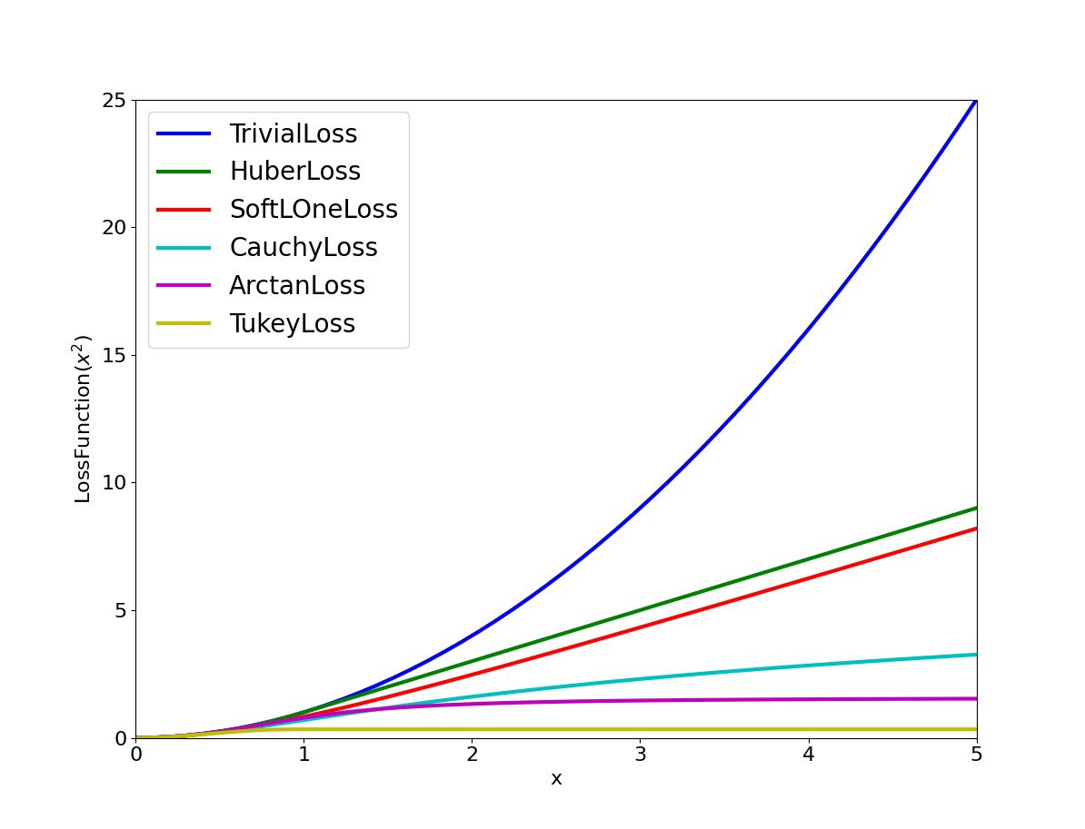
Shape of the various common loss functions.
-
class TrivialLoss
- \[\rho(s) = s\]
-
class HuberLoss
- \[\begin{split}\rho(s) = \begin{cases} s & s \le 1\\ 2 \sqrt{s} - 1 & s > 1 \end{cases}\end{split}\]
-
class SoftLOneLoss
- \[\rho(s) = 2 (\sqrt{1+s} - 1)\]
-
class CauchyLoss
- \[\rho(s) = \log(1 + s)\]
-
class ArctanLoss
- \[\rho(s) = \arctan(s)\]
-
class TolerantLoss
- \[\rho(s,a,b) = b \log(1 + e^{(s - a) / b}) - b \log(1 + e^{-a / b})\]
-
class TukeyLoss
- \[\begin{split}\rho(s) = \begin{cases} \frac{1}{3} (1 - (1 - s)^3) & s \le 1\\ \frac{1}{3} & s > 1 \end{cases}\end{split}\]
-
class ComposedLoss
Given two loss functions
fandg, implements the loss functionh(s) = f(g(s)).class ComposedLoss : public LossFunction { public: explicit ComposedLoss(const LossFunction* f, Ownership ownership_f, const LossFunction* g, Ownership ownership_g); };
-
class ScaledLoss
Sometimes you want to simply scale the output value of the robustifier. For example, you might want to weight different error terms differently (e.g., weight pixel reprojection errors differently from terrain errors).
Given a loss function \(\rho(s)\) and a scalar \(a\),
ScaledLossimplements the function \(a \rho(s)\).Since we treat a
nullptrLoss function as the Identity loss function, \(rho\) =nullptr: is a valid input and will result in the input being scaled by \(a\). This provides a simple way of implementing a scaled ResidualBlock.
-
class LossFunctionWrapper
Sometimes after the optimization problem has been constructed, we wish to mutate the scale of the loss function. For example, when performing estimation from data which has substantial outliers, convergence can be improved by starting out with a large scale, optimizing the problem and then reducing the scale. This can have better convergence behavior than just using a loss function with a small scale.
This templated class allows the user to implement a loss function whose scale can be mutated after an optimization problem has been constructed, e.g,
Problem problem;

// Add parameter blocks

auto* cost_function =
    new AutoDiffCostFunction<UW_Camera_Mapper, 2, 9, 3>(feature_x, feature_y);

LossFunctionWrapper* loss_function(new HuberLoss(1.0), TAKE_OWNERSHIP);
problem.AddResidualBlock(cost_function, loss_function, parameters);

Solver::Options options;
Solver::Summary summary;
Solve(options, &problem, &summary);

loss_function->Reset(new HuberLoss(1.0), TAKE_OWNERSHIP);
Solve(options, &problem, &summary);
Theory
Let us consider a problem with a single parameter block.
Then, the robustified gradient and the Gauss-Newton Hessian are
where the terms involving the second derivatives of \(f(x)\) have been ignored. Note that \(H(x)\) is indefinite if \(\rho''f(x)^\top f(x) + \frac{1}{2}\rho' < 0\). If this is not the case, then its possible to re-weight the residual and the Jacobian matrix such that the robustified Gauss-Newton step corresponds to an ordinary linear least squares problem.
Let \(\alpha\) be a root of
Then, define the rescaled residual and Jacobian as
In the case \(2 \rho''\left\|f(x)\right\|^2 + \rho' \lesssim 0\), we limit \(\alpha \le 1- \epsilon\) for some small \(\epsilon\). For more details see [Triggs].
With this simple rescaling, one can apply any Jacobian based non-linear least squares algorithm to robustified non-linear least squares problems.
While the theory described above is elegant, in practice we observe that using the Triggs correction when \(\rho'' > 0\) leads to poor performance, so we upper bound it by zero. For more details see corrector.cc
Manifold
-
class Manifold
In sensor fusion problems, we often have to model quantities that live in spaces known as Manifolds, for example the rotation/orientation of a sensor that is represented by a Quaternion.
Manifolds are spaces which locally look like Euclidean spaces. More precisely, at each point on the manifold there is a linear space that is tangent to the manifold. It has dimension equal to the intrinsic dimension of the manifold itself, which is less than or equal to the ambient space in which the manifold is embedded.
For example, the tangent space to a point on a sphere in three dimensions is the two dimensional plane that is tangent to the sphere at that point. There are two reasons tangent spaces are interesting:
They are Eucliean spaces so the usual vector space operations apply there, which makes numerical operations easy.
Movements in the tangent space translate into movements along the manifold. Movements perpendicular to the tangent space do not translate into movements on the manifold.
However, moving along the 2 dimensional plane tangent to the sphere and projecting back onto the sphere will move you away from the point you started from but moving along the normal at the same point and the projecting back onto the sphere brings you back to the point.
Besides the mathematical niceness, modeling manifold valued quantities correctly and paying attention to their geometry has practical benefits too:
It naturally constrains the quantity to the manifold throughout the optimization, freeing the user from hacks like quaternion normalization.
It reduces the dimension of the optimization problem to its natural size. For example, a quantity restricted to a line is a one dimensional object regardless of the dimension of the ambient space in which this line lives.
Working in the tangent space reduces not just the computational complexity of the optimization algorithm, but also improves the numerical behaviour of the algorithm.
A basic operation one can perform on a manifold is the \(\boxplus\) operation that computes the result of moving along \(\delta\) in the tangent space at \(x\), and then projecting back onto the manifold that \(x\) belongs to. Also known as a Retraction, \(\boxplus\) is a generalization of vector addition in Euclidean spaces.
The inverse of \(\boxplus\) is \(\boxminus\), which given two points \(y\) and \(x\) on the manifold computes the tangent vector \(\Delta\) at \(x\) s.t. \(\boxplus(x, \Delta) = y\).
Let us now consider two examples.
The Euclidean space \(\mathbb{R}^n\) is the simplest example of a manifold. It has dimension \(n\) (and so does its tangent space) and \(\boxplus\) and \(\boxminus\) are the familiar vector sum and difference operations.
A more interesting case is the case \(SO(3)\), the special orthogonal group in three dimensions - the space of \(3\times3\) rotation matrices. \(SO(3)\) is a three dimensional manifold embedded in \(\mathbb{R}^9\) or \(\mathbb{R}^{3\times 3}\). So points on \(SO(3)\) are represented using 9 dimensional vectors or \(3\times 3\) matrices, and points in its tangent spaces are represented by 3 dimensional vectors.
For \(SO(3)\), \(\boxplus\) and \(\boxminus\) are defined in terms of the matrix \(\exp\) and \(\log\) operations as follows:
Given a 3-vector \(\Delta = [\begin{matrix}p,&q,&r\end{matrix}]\), we have
where,
Given \(x \in SO(3)\), we have
where,
Then,
For \(\boxplus\) and \(\boxminus\) to be mathematically consistent, the following identities must be satisfied at all points \(x\) on the manifold:
\(\boxplus(x, 0) = x\). This ensures that the tangent space is centered at \(x\), and the zero vector is the identity element.
For all \(y\) on the manifold, \(\boxplus(x, \boxminus(y,x)) = y\). This ensures that any \(y\) can be reached from \(x\).
For all \(\Delta\), \(\boxminus(\boxplus(x, \Delta), x) = \Delta\). This ensures that \(\boxplus\) is an injective (one-to-one) map.
For all \(\Delta_1, \Delta_2\ |\boxminus(\boxplus(x, \Delta_1), \boxplus(x, \Delta_2)) \leq |\Delta_1 - \Delta_2|\). Allows us to define a metric on the manifold.
Additionally we require that \(\boxplus\) and \(\boxminus\) be sufficiently smooth. In particular they need to be differentiable everywhere on the manifold.
For more details, please see [Hertzberg]
The Manifold interface allows the user to define a manifold
for the purposes optimization by implementing Plus and Minus
operations and their derivatives (corresponding naturally to
\(\boxplus\) and \(\boxminus\)).
class Manifold {
 public:
  virtual ~Manifold();
  virtual int AmbientSize() const = 0;
  virtual int TangentSize() const = 0;
  virtual bool Plus(const double* x,
                    const double* delta,
                    double* x_plus_delta) const = 0;
  virtual bool PlusJacobian(const double* x, double* jacobian) const = 0;
  virtual bool RightMultiplyByPlusJacobian(const double* x,
                                           const int num_rows,
                                           const double* ambient_matrix,
                                           double* tangent_matrix) const;
  virtual bool Minus(const double* y,
                     const double* x,
                     double* y_minus_x) const = 0;
  virtual bool MinusJacobian(const double* x, double* jacobian) const = 0;
};
-
int Manifold::AmbientSize() const;
Dimension of the ambient space in which the manifold is embedded.
-
bool Plus(const double *x, const double *delta, double *x_plus_delta) const;
Implements the \(\boxplus(x,\Delta)\) operation for the manifold.
A generalization of vector addition in Euclidean space,
Pluscomputes the result of moving alongdeltain the tangent space atx, and then projecting back onto the manifold thatxbelongs to.xandx_plus_deltaareManifold::AmbientSize()vectors.deltais aManifold::TangentSize()vector.Return value indicates if the operation was successful or not.
-
bool PlusJacobian(const double *x, double *jacobian) const;
Compute the derivative of \(\boxplus(x, \Delta)\) w.r.t \(\Delta\) at \(\Delta = 0\), i.e. \((D_2 \boxplus)(x, 0)\).
jacobianis a row-majorManifold::AmbientSize()\(\times\)Manifold::TangentSize()matrix.Return value indicates whether the operation was successful or not.
-
bool RightMultiplyByPlusJacobian(const double *x, const int num_rows, const double *ambient_matrix, double *tangent_matrix) const;
tangent_matrix=ambient_matrix\(\times\) plus_jacobian.ambient_matrixis a row-majornum_rows\(\times\)Manifold::AmbientSize()matrix.tangent_matrixis a row-majornum_rows\(\times\)Manifold::TangentSize()matrix.Return value indicates whether the operation was successful or not.
This function is only used by the
GradientProblemSolver, where the dimension of the parameter block can be large and it may be more efficient to compute this product directly rather than first evaluating the Jacobian into a matrix and then doing a matrix vector product.Because this is not an often used function, we provide a default implementation for convenience. If performance becomes an issue then the user should consider implementing a specialization.
-
bool Minus(const double *y, const double *x, double *y_minus_x) const;
Implements \(\boxminus(y,x)\) operation for the manifold.
A generalization of vector subtraction in Euclidean spaces, given two points
xandyon the manifold,Minuscomputes the change toxin the tangent space atx, that will take it toy.xandyareManifold::AmbientSize()vectors.y_minus_xis a :Manifold::TangentSize()vector.Return value indicates if the operation was successful or not.
-
bool MinusJacobian(const double *x, double *jacobian) const = 0;
Compute the derivative of \(\boxminus(y, x)\) w.r.t \(y\) at \(y = x\), i.e \((D_1 \boxminus) (x, x)\).
jacobianis a row-majorManifold::TangentSize()\(\times\)Manifold::AmbientSize()matrix.Return value indicates whether the operation was successful or not.
Ceres Solver ships with a number of commonly used instances of
Manifold.
For Lie Groups, a great place to find high quality implementations is the Sophus library developed by Hauke Strasdat and his collaborators.
EuclideanManifold
-
class EuclideanManifold
EuclideanManifold as the name implies represents a Euclidean
space, where the \(\boxplus\) and \(\boxminus\) operations are
the usual vector addition and subtraction.
By default parameter blocks are assumed to be Euclidean, so there is
no need to use this manifold on its own. It is provided for the
purpose of testing and for use in combination with other manifolds
using ProductManifold.
The class works with dynamic and static ambient space dimensions. If the ambient space dimensions is known at compile time use
EuclideanManifold<3> manifold;
If the ambient space dimensions is not known at compile time the template parameter needs to be set to ceres::DYNAMIC and the actual dimension needs to be provided as a constructor argument:
EuclideanManifold<ceres::DYNAMIC> manifold(ambient_dim);
SubsetManifold
-
class SubsetManifold
Suppose \(x\) is a two dimensional vector, and the user wishes to hold the first coordinate constant. Then, \(\Delta\) is a scalar and \(\boxplus\) is defined as
and given two, two-dimensional vectors \(x\) and \(y\) with the same first coordinate, \(\boxminus\) is defined as:
SubsetManifold generalizes this construction to hold
any part of a parameter block constant by specifying the set of
coordinates that are held constant.
Note
It is legal to hold all coordinates of a parameter block to
constant using a SubsetManifold. It is the same as calling
Problem::SetParameterBlockConstant() on that parameter block.
ProductManifold
-
class ProductManifold
In cases, where a parameter block is the Cartesian product of a number
of manifolds and you have the manifold of the individual
parameter blocks available, ProductManifold can be used to
construct a Manifold of the Cartesian product.
For the case of the rigid transformation, where say you have a parameter block of size 7, where the first four entries represent the rotation as a quaternion, and the next three the translation, a manifold can be constructed as:
ProductManifold<QuaternionManifold, EuclideanManifold<3>> se3;
Manifolds can be copied and moved to ProductManifold:
SubsetManifold manifold1(5, {2});
SubsetManifold manifold2(3, {0, 1});
ProductManifold<SubsetManifold, SubsetManifold> manifold(manifold1,
                                                         manifold2);
In advanced use cases, manifolds can be dynamically allocated and passed as (smart) pointers:
ProductManifold<std::unique_ptr<QuaternionManifold>, EuclideanManifold<3>> se3
     {std::make_unique<QuaternionManifold>(), EuclideanManifold<3>{}};
The template parameters can also be left out as they are deduced automatically making the initialization much simpler:
ProductManifold se3{QuaternionManifold{}, EuclideanManifold<3>{}};
QuaternionManifold
-
class QuaternionManifold
Note
If you are using Eigen quaternions, then you should use
EigenQuaternionManifold instead because Eigen uses a
different memory layout for its Quaternions.
Manifold for a Hamilton Quaternion. Quaternions are a three dimensional manifold represented as unit norm 4-vectors, i.e.
is the ambient space representation. Here \(q_0\) is the scalar part. \(q_1\) is the coefficient of \(i\), \(q_2\) is the coefficient of \(j\), and \(q_3\) is the coefficient of \(k\). Where:
The tangent space is three dimensional and the \(\boxplus\) and \(\boxminus\) operators are defined in term of \(\exp\) and \(\log\) operations.
Where \(\otimes\) is the Quaternion product and since \(x\) is a unit quaternion, \(x^{-1} = [\begin{matrix} q_0,& -q_1,& -q_2,& -q_3\end{matrix}]\). Given a vector \(\Delta \in \mathbb{R}^3\),
and given a unit quaternion \(q = \left [\begin{matrix}q_0,& q_1,& q_2,& q_3\end{matrix}\right]\)
EigenQuaternionManifold
-
class EigenQuaternionManifold
Implements the quaternion manifold for Eigen’s
representation of the Hamilton quaternion. Geometrically it is exactly
the same as the QuaternionManifold defined above. However,
Eigen uses a different internal memory layout for the elements of the
quaternion than what is commonly used. It stores the quaternion in
memory as \([q_1, q_2, q_3, q_0]\) or \([x, y, z, w]\) where
the real (scalar) part is last.
Since Ceres operates on parameter blocks which are raw double pointers this difference is important and requires a different manifold.
SphereManifold
-
class SphereManifold
This provides a manifold on a sphere meaning that the norm of the vector stays the same. Such cases often arises in Structure for Motion problems. One example where they are used is in representing points whose triangulation is ill-conditioned. Here it is advantageous to use an over-parameterization since homogeneous vectors can represent points at infinity.
The ambient space dimension is required to be greater than 1.
The class works with dynamic and static ambient space dimensions. If the ambient space dimensions is known at compile time use
SphereManifold<3> manifold;
If the ambient space dimensions is not known at compile time the template parameter needs to be set to ceres::DYNAMIC and the actual dimension needs to be provided as a constructor argument:
SphereManifold<ceres::DYNAMIC> manifold(ambient_dim);
For more details, please see Section B.2 (p.25) in [Hertzberg]
LineManifold
-
class LineManifold
This class provides a manifold for lines, where the line is defined using an origin point and a direction vector. So the ambient size needs to be two times the dimension of the space in which the line lives. The first half of the parameter block is interpreted as the origin point and the second half as the direction. This manifold is a special case of the Affine Grassmannian manifold for the case \(\operatorname{Graff}_1(R^n)\).
Note that this is a manifold for a line, rather than a point constrained to lie on a line. It is useful when one wants to optimize over the space of lines. For example, given \(n\) distinct points in 3D (measurements) we want to find the line that minimizes the sum of squared distances to all the points.
AutoDiffManifold
-
class AutoDiffManifold
Create a Manifold with Jacobians computed via automatic
differentiation.
To get an auto differentiated manifold, you must define a Functor with
templated Plus and Minus functions that compute:
x_plus_delta = Plus(x, delta);
y_minus_x    = Minus(y, x);
Where, x, y and x_plus_delta are vectors on the manifold in
the ambient space (so they are kAmbientSize vectors) and
delta, y_minus_x are vectors in the tangent space (so they are
kTangentSize vectors).
The Functor should have the signature:
struct Functor {
 template <typename T>
 bool Plus(const T* x, const T* delta, T* x_plus_delta) const;

 template <typename T>
 bool Minus(const T* y, const T* x, T* y_minus_x) const;
};
Observe that the Plus and Minus operations are templated on
the parameter T. The autodiff framework substitutes appropriate
Jet objects for T in order to compute the derivative when
necessary. This is the same mechanism that is used to compute
derivatives when using AutoDiffCostFunction.
Plus and Minus should return true if the computation is
successful and false otherwise, in which case the result will not be
used.
Given this Functor, the corresponding Manifold can be constructed as:
AutoDiffManifold<Functor, kAmbientSize, kTangentSize> manifold;
Note
The following is only used for illustration purposes. Ceres Solver
ships with an optimized, production grade QuaternionManifold
implementation.
As a concrete example consider the case of Quaternions. Quaternions form a three
dimensional manifold embedded in \(\mathbb{R}^4\), i.e. they have
an ambient dimension of 4 and their tangent space has dimension 3. The
following Functor defines the Plus and Minus operations on the
Quaternion manifold. It assumes that the quaternions are laid out as
[w,x,y,z] in memory, i.e. the real or scalar part is the first
coordinate.
struct QuaternionFunctor {
  template <typename T>
  bool Plus(const T* x, const T* delta, T* x_plus_delta) const {
    const T squared_norm_delta =
        delta[0] * delta[0] + delta[1] * delta[1] + delta[2] * delta[2];

    T q_delta[4];
    if (squared_norm_delta > T(0.0)) {
      T norm_delta = sqrt(squared_norm_delta);
      const T sin_delta_by_delta = sin(norm_delta) / norm_delta;
      q_delta[0] = cos(norm_delta);
      q_delta[1] = sin_delta_by_delta * delta[0];
      q_delta[2] = sin_delta_by_delta * delta[1];
      q_delta[3] = sin_delta_by_delta * delta[2];
    } else {
      // We do not just use q_delta = [1,0,0,0] here because that is a
      // constant and when used for automatic differentiation will
      // lead to a zero derivative. Instead we take a first order
      // approximation and evaluate it at zero.
      q_delta[0] = T(1.0);
      q_delta[1] = delta[0];
      q_delta[2] = delta[1];
      q_delta[3] = delta[2];
    }

    QuaternionProduct(q_delta, x, x_plus_delta);
    return true;
  }

  template <typename T>
  bool Minus(const T* y, const T* x, T* y_minus_x) const {
    T minus_x[4] = {x[0], -x[1], -x[2], -x[3]};
    T ambient_y_minus_x[4];
    QuaternionProduct(y, minus_x, ambient_y_minus_x);
    T u_norm = sqrt(ambient_y_minus_x[1] * ambient_y_minus_x[1] +
                    ambient_y_minus_x[2] * ambient_y_minus_x[2] +
                    ambient_y_minus_x[3] * ambient_y_minus_x[3]);
    if (u_norm > 0.0) {
      T theta = atan2(u_norm, ambient_y_minus_x[0]);
      y_minus_x[0] = theta * ambient_y_minus_x[1] / u_norm;
      y_minus_x[1] = theta * ambient_y_minus_x[2] / u_norm;
      y_minus_x[2] = theta * ambient_y_minus_x[3] / u_norm;
    } else {
      We do not use [0,0,0] here because even though the value part is
      a constant, the derivative part is not.
      y_minus_x[0] = ambient_y_minus_x[1];
      y_minus_x[1] = ambient_y_minus_x[2];
      y_minus_x[2] = ambient_y_minus_x[3];
    }
    return true;
  }
};
Then given this struct, the auto differentiated Quaternion Manifold can now be constructed as
Manifold* manifold = new AutoDiffManifold<QuaternionFunctor, 4, 3>;
Problem
-
class Problem
Problemholds the robustified bounds constrained non-linear least squares problem (1). To create a least squares problem, use theProblem::AddResidalBlock()andProblem::AddParameterBlock()methods.For example a problem containing 3 parameter blocks of sizes 3, 4 and 5 respectively and two residual blocks of size 2 and 6:
double x1[] = { 1.0, 2.0, 3.0 };
double x2[] = { 1.0, 2.0, 3.0, 5.0 };
double x3[] = { 1.0, 2.0, 3.0, 6.0, 7.0 };

Problem problem;
problem.AddResidualBlock(new MyUnaryCostFunction(...), x1);
problem.AddResidualBlock(new MyBinaryCostFunction(...), x2, x3);
Problem::AddResidualBlock()as the name implies, adds a residual block to the problem. It adds aCostFunction, an optionalLossFunctionand connects theCostFunctionto a set of parameter block.The cost function carries with it information about the sizes of the parameter blocks it expects. The function checks that these match the sizes of the parameter blocks listed in
parameter_blocks. The program aborts if a mismatch is detected.loss_functioncan benullptr, in which case the cost of the term is just the squared norm of the residuals.The user has the option of explicitly adding the parameter blocks using
Problem::AddParameterBlock(). This causes additional correctness checking; however,Problem::AddResidualBlock()implicitly adds the parameter blocks if they are not present, so callingProblem::AddParameterBlock()explicitly is not required.Problem::AddParameterBlock()explicitly adds a parameter block to theProblem. Optionally it allows the user to associate aManifoldobject with the parameter block too. Repeated calls with the same arguments are ignored. Repeated calls with the same double pointer but a different size results in undefined behavior.You can set any parameter block to be constant using
Problem::SetParameterBlockConstant()and undo this usingSetParameterBlockVariable().In fact you can set any number of parameter blocks to be constant, and Ceres is smart enough to figure out what part of the problem you have constructed depends on the parameter blocks that are free to change and only spends time solving it. So for example if you constructed a problem with a million parameter blocks and 2 million residual blocks, but then set all but one parameter blocks to be constant and say only 10 residual blocks depend on this one non-constant parameter block. Then the computational effort Ceres spends in solving this problem will be the same if you had defined a problem with one parameter block and 10 residual blocks.
Ownership
Problemby default takes ownership of thecost_function,loss_functionandmanifoldpointers. These objects remain live for the life of theProblem. If the user wishes to keep control over the destruction of these objects, then they can do this by setting the corresponding enums in theProblem::Optionsstruct.Note that even though the Problem takes ownership of objects,
cost_functionandloss_function, it does not preclude the user from re-using them in another residual block. Similarly the samemanifoldobject can be used with multiple parameter blocks. The destructor takes care to call delete on each owned object exactly once.
-
Ownership Problem::Options::cost_function_ownership
Default:
TAKE_OWNERSHIPThis option controls whether the Problem object owns the cost functions.
If set to
TAKE_OWNERSHIP, then the problem object will delete the cost functions on destruction. The destructor is careful to delete the pointers only once, since sharing cost functions is allowed.
-
Ownership Problem::Options::loss_function_ownership
Default:
TAKE_OWNERSHIPThis option controls whether the Problem object owns the loss functions.
If set to
TAKE_OWNERSHIP, then the problem object will delete the loss functions on destruction. The destructor is careful to delete the pointers only once, since sharing loss functions is allowed.
-
Ownership Problem::Options::manifold_ownership
Default:
TAKE_OWNERSHIPThis option controls whether the Problem object owns the manifolds.
If set to
TAKE_OWNERSHIP, then the problem object will delete the manifolds on destruction. The destructor is careful to delete the pointers only once, since sharing manifolds is allowed.
-
bool Problem::Options::enable_fast_removal
Default:
falseIf true, trades memory for faster
Problem::RemoveResidualBlock()andProblem::RemoveParameterBlock()operations.By default,
Problem::RemoveParameterBlock()andProblem::RemoveResidualBlock()take time proportional to the size of the entire problem. If you only ever remove parameters or residuals from the problem occasionally, this might be acceptable. However, if you have memory to spare, enable this option to makeProblem::RemoveParameterBlock()take time proportional to the number of residual blocks that depend on it, andProblem::RemoveResidualBlock()take (on average) constant time.The increase in memory usage is twofold: an additional hash set per parameter block containing all the residuals that depend on the parameter block; and a hash set in the problem containing all residuals.
-
bool Problem::Options::disable_all_safety_checks
Default: false
By default, Ceres performs a variety of safety checks when constructing the problem. There is a small but measurable performance penalty to these checks, typically around 5% of construction time. If you are sure your problem construction is correct, and 5% of the problem construction time is truly an overhead you want to avoid, then you can set disable_all_safety_checks to true.
Warning
Do not set this to true, unless you are absolutely sure of what you are doing.
-
Context *Problem::Options::context
Default:
nullptrA Ceres global context to use for solving this problem. This may help to reduce computation time as Ceres can reuse expensive objects to create. The context object can be nullptr, in which case Ceres may create one.
Ceres does NOT take ownership of the pointer.
-
EvaluationCallback *Problem::Options::evaluation_callback
Default:
nullptrUsing this callback interface, Ceres will notify you when it is about to evaluate the residuals or Jacobians.
If an
evaluation_callbackis present, Ceres will update the user’s parameter blocks to the values that will be used when callingCostFunction::Evaluate()before callingEvaluationCallback::PrepareForEvaluation(). One can then use this callback to share (or cache) computation between cost functions by doing the shared computation inEvaluationCallback::PrepareForEvaluation()before Ceres callsCostFunction::Evaluate().Problem does NOT take ownership of the callback.
Note
Evaluation callbacks are incompatible with inner iterations. So calling Solve with
Solver::Options::use_inner_iterationsset totrueon aProblemwith a non-null evaluation callback is an error.
-
ResidualBlockId Problem::AddResidualBlock(CostFunction *cost_function, LossFunction *loss_function, const std::vector<double*> parameter_blocks)
-
template<typename Ts...>
ResidualBlockId Problem::AddResidualBlock(CostFunction *cost_function, LossFunction *loss_function, double *x0, Ts... xs)¶ Add a residual block to the overall cost function. The cost function carries with it information about the sizes of the parameter blocks it expects. The function checks that these match the sizes of the parameter blocks listed in parameter_blocks. The program aborts if a mismatch is detected. loss_function can be
nullptr, in which case the cost of the term is just the squared norm of the residuals.The parameter blocks may be passed together as a
vector<double*>, ordouble*pointers.The user has the option of explicitly adding the parameter blocks using AddParameterBlock. This causes additional correctness checking; however, AddResidualBlock implicitly adds the parameter blocks if they are not present, so calling AddParameterBlock explicitly is not required.
The Problem object by default takes ownership of the cost_function and loss_function pointers. These objects remain live for the life of the Problem object. If the user wishes to keep control over the destruction of these objects, then they can do this by setting the corresponding enums in the Options struct.
Note
Even though the Problem takes ownership of
cost_functionandloss_function, it does not preclude the user from re-using them in another residual block. The destructor takes care to call delete on each cost_function or loss_function pointer only once, regardless of how many residual blocks refer to them.Example usage:
double x1[] = {1.0, 2.0, 3.0};
double x2[] = {1.0, 2.0, 5.0, 6.0};
double x3[] = {3.0, 6.0, 2.0, 5.0, 1.0};
std::vector<double*> v1;
v1.push_back(x1);
std::vector<double*> v2;
v2.push_back(x2);
v2.push_back(x1);

Problem problem;

problem.AddResidualBlock(new MyUnaryCostFunction(...), nullptr, x1);
problem.AddResidualBlock(new MyBinaryCostFunction(...), nullptr, x2, x1);
problem.AddResidualBlock(new MyUnaryCostFunction(...), nullptr, v1);
problem.AddResidualBlock(new MyBinaryCostFunction(...), nullptr, v2);
-
void Problem::AddParameterBlock(double *values, int size, Manifold *manifold)
Add a parameter block with appropriate size and Manifold to the problem. It is okay for
manifoldto benullptr.Repeated calls with the same arguments are ignored. Repeated calls with the same double pointer but a different size results in a crash (unless
Solver::Options::disable_all_safety_checksis set to true).Repeated calls with the same double pointer and size but different
Manifoldis equivalent to calling SetManifold(manifold), i.e., any previously associatedManifoldobject will be replaced with the manifold.
-
void Problem::AddParameterBlock(double *values, int size)
Add a parameter block with appropriate size and parameterization to the problem. Repeated calls with the same arguments are ignored. Repeated calls with the same double pointer but a different size results in undefined behavior.
-
void Problem::RemoveResidualBlock(ResidualBlockId residual_block)
Remove a residual block from the problem.
Since residual blocks are allowed to share cost function and loss function objects, Ceres Solver uses a reference counting mechanism. So when a residual block is deleted, the reference count for the corresponding cost function and loss function objects are decreased and when this count reaches zero, they are deleted.
If
Problem::Options::enable_fast_removalistrue, then the removal is fast (almost constant time). Otherwise it is linear, requiring a scan of the entire problem.Removing a residual block has no effect on the parameter blocks that the problem depends on.
Warning
Removing a residual or parameter block will destroy the implicit ordering, rendering the jacobian or residuals returned from the solver uninterpretable. If you depend on the evaluated jacobian, do not use remove! This may change in a future release. Hold the indicated parameter block constant during optimization.
-
void Problem::RemoveParameterBlock(const double *values)
Remove a parameter block from the problem. Any residual blocks that depend on the parameter are also removed, as described above in
RemoveResidualBlock().The manifold of the parameter block, if it exists, will persist until the deletion of the problem.
If
Problem::Options::enable_fast_removalistrue, then the removal is fast (almost constant time). Otherwise, removing a parameter block will scan the entire Problem.Warning
Removing a residual or parameter block will destroy the implicit ordering, rendering the jacobian or residuals returned from the solver uninterpretable. If you depend on the evaluated jacobian, do not use remove! This may change in a future release.
-
void Problem::SetParameterBlockConstant(const double *values)
Hold the indicated parameter block constant during optimization.
-
void Problem::SetParameterBlockVariable(double *values)
Allow the indicated parameter to vary during optimization.
-
bool Problem::IsParameterBlockConstant(const double *values) const
Returns
trueif a parameter block is set constant, and false otherwise. A parameter block may be set constant in two ways: either by callingSetParameterBlockConstantor by associating aManifoldwith a zero dimensional tangent space with it.
-
void SetManifold(double *values, Manifold *manifold);
Set the
Manifoldfor the parameter block. CallingProblem::SetManifold()withnullptrwill clear any previously setManifoldfor the parameter block.Repeated calls will result in any previously associated
Manifoldobject to be replaced withmanifold.manifoldis owned byProblemby default (SeeProblem::Optionsto override this behaviour).It is acceptable to set the same
Manifoldfor multiple parameter blocks.
-
const Manifold *GetManifold(const double *values) const;
Get the
Manifoldobject associated with this parameter block.If there is no
Manifoldobject associated with the parameter block, thennullptris returned.
-
bool HasManifold(const double *values) const;
Returns
trueif aManifoldis associated with this parameter block,falseotherwise.
-
void Problem::SetParameterLowerBound(double *values, int index, double lower_bound)
Set the lower bound for the parameter at position index in the parameter block corresponding to values. By default the lower bound is
-std::numeric_limits<double>::max(), which is treated by the solver as the same as \(-\infty\).
-
void Problem::SetParameterUpperBound(double *values, int index, double upper_bound)
Set the upper bound for the parameter at position index in the parameter block corresponding to values. By default the value is
std::numeric_limits<double>::max(), which is treated by the solver as the same as \(\infty\).
-
double Problem::GetParameterLowerBound(const double *values, int index)
Get the lower bound for the parameter with position index. If the parameter is not bounded by the user, then its lower bound is
-std::numeric_limits<double>::max().
-
double Problem::GetParameterUpperBound(const double *values, int index)
Get the upper bound for the parameter with position index. If the parameter is not bounded by the user, then its upper bound is
std::numeric_limits<double>::max().
-
int Problem::NumParameterBlocks() const
Number of parameter blocks in the problem. Always equals parameter_blocks().size() and parameter_block_sizes().size().
-
int Problem::NumParameters() const
The size of the parameter vector obtained by summing over the sizes of all the parameter blocks.
-
int Problem::NumResidualBlocks() const
Number of residual blocks in the problem. Always equals residual_blocks().size().
-
int Problem::NumResiduals() const
The size of the residual vector obtained by summing over the sizes of all of the residual blocks.
-
int Problem::ParameterBlockTangentSize(const double *values) const
The dimension of the tangent space of the
Manifoldfor the parameter block. If there is noManifoldassociated with this parameter block, thenParameterBlockTangentSize = ParameterBlockSize.
-
bool Problem::HasParameterBlock(const double *values) const
Is the given parameter block present in the problem or not?
-
void Problem::GetParameterBlocks(std::vector<double*> *parameter_blocks) const
Fills the passed
parameter_blocksvector with pointers to the parameter blocks currently in the problem. After this call,parameter_block.size() == NumParameterBlocks.
-
void Problem::GetResidualBlocks(std::vector<ResidualBlockId> *residual_blocks) const
Fills the passed residual_blocks vector with pointers to the residual blocks currently in the problem. After this call, residual_blocks.size() == NumResidualBlocks.
-
void Problem::GetParameterBlocksForResidualBlock(const ResidualBlockId residual_block, std::vector<double*> *parameter_blocks) const
Get all the parameter blocks that depend on the given residual block.
-
void Problem::GetResidualBlocksForParameterBlock(const double *values, std::vector<ResidualBlockId> *residual_blocks) const
Get all the residual blocks that depend on the given parameter block.
If
Problem::Options::enable_fast_removalistrue, then getting the residual blocks is fast and depends only on the number of residual blocks. Otherwise, getting the residual blocks for a parameter block will scan the entire problem.
-
const CostFunction *Problem::GetCostFunctionForResidualBlock(const ResidualBlockId residual_block) const
Get the
CostFunctionfor the given residual block.
-
const LossFunction *Problem::GetLossFunctionForResidualBlock(const ResidualBlockId residual_block) const
Get the
LossFunctionfor the given residual block.
-
bool EvaluateResidualBlock(ResidualBlockId residual_block_id, bool apply_loss_function, double *cost, double *residuals, double **jacobians) const
Evaluates the residual block, storing the scalar cost in
cost, the residual components inresiduals, and the jacobians between the parameters and residuals injacobians[i], in row-major order.If
residualsisnullptr, the residuals are not computed.If
jacobiansisnullptr, no Jacobians are computed. Ifjacobians[i]isnullptr, then the Jacobian for that parameter block is not computed.It is not okay to request the Jacobian w.r.t a parameter block that is constant.
The return value indicates the success or failure. Even if the function returns false, the caller should expect the output memory locations to have been modified.
The returned cost and jacobians have had robustification and
Manifoldapplied already; for example, the jacobian for a 4-dimensional quaternion parameter using theQuaternionManifoldisnum_residuals x 3instead ofnum_residuals x 4.apply_loss_functionas the name implies allows the user to switch the application of the loss function on and off.Note
If an
EvaluationCallbackis associated with the problem, then itsEvaluationCallback::PrepareForEvaluation()method will be called every time this method is called with new_point = true. This conservatively assumes that the user may have changed the parameter values since the previous call to evaluate / solve. For improved efficiency, and only if you know that the parameter values have not changed between calls, seeProblem::EvaluateResidualBlockAssumingParametersUnchanged().
-
bool EvaluateResidualBlockAssumingParametersUnchanged(ResidualBlockId residual_block_id, bool apply_loss_function, double *cost, double *residuals, double **jacobians) const
Same as
Problem::EvaluateResidualBlock()except that if anEvaluationCallbackis associated with the problem, then itsEvaluationCallback::PrepareForEvaluation()method will be called every time this method is called with new_point = false.This means, if an
EvaluationCallbackis associated with the problem then it is the user’s responsibility to callEvaluationCallback::PrepareForEvaluation()before calling this method if necessary, i.e. iff the parameter values have been changed since the last call to evaluate / solve.’This is because, as the name implies, we assume that the parameter blocks did not change since the last time
EvaluationCallback::PrepareForEvaluation()was called (viaSolve(),Problem::Evaluate()orProblem::EvaluateResidualBlock()).
-
bool Problem::Evaluate(const Problem::EvaluateOptions &options, double *cost, std::vector<double> *residuals, std::vector<double> *gradient, CRSMatrix *jacobian)
Evaluate a
Problem. Any of the output pointers can benullptr. Which residual blocks and parameter blocks are used is controlled by theProblem::EvaluateOptionsstruct below.Note
The evaluation will use the values stored in the memory locations pointed to by the parameter block pointers used at the time of the construction of the problem, for example in the following code:
Problem problem;
double x = 1;
problem.Add(new MyCostFunction, nullptr, &x);

double cost = 0.0;
problem.Evaluate(Problem::EvaluateOptions(), &cost, nullptr, nullptr, nullptr);
The cost is evaluated at x = 1. If you wish to evaluate the problem at x = 2, then
x = 2;
problem.Evaluate(Problem::EvaluateOptions(), &cost, nullptr, nullptr, nullptr);
is the way to do so.
Note
If no
Manifoldare used, then the size of the gradient vector is the sum of the sizes of all the parameter blocks. If a parameter block has a manifold then it contributes “TangentSize” entries to the gradient vector.Note
This function cannot be called while the problem is being solved, for example it cannot be called from an
IterationCallbackat the end of an iteration during a solve.Note
If an EvaluationCallback is associated with the problem, then its PrepareForEvaluation method will be called everytime this method is called with
new_point = true.
-
class Problem::EvaluateOptions
Options struct that is used to control
Problem::Evaluate().
-
std::vector<double*> Problem::EvaluateOptions::parameter_blocks
The set of parameter blocks for which evaluation should be performed. This vector determines the order in which parameter blocks occur in the gradient vector and in the columns of the jacobian matrix. If parameter_blocks is empty, then it is assumed to be equal to a vector containing ALL the parameter blocks. Generally speaking the ordering of the parameter blocks in this case depends on the order in which they were added to the problem and whether or not the user removed any parameter blocks.
NOTE This vector should contain the same pointers as the ones used to add parameter blocks to the Problem. These parameter block should NOT point to new memory locations. Bad things will happen if you do.
-
std::vector<ResidualBlockId> Problem::EvaluateOptions::residual_blocks
The set of residual blocks for which evaluation should be performed. This vector determines the order in which the residuals occur, and how the rows of the jacobian are ordered. If residual_blocks is empty, then it is assumed to be equal to the vector containing all the residual blocks.
-
bool Problem::EvaluateOptions::apply_loss_function
Even though the residual blocks in the problem may contain loss functions, setting apply_loss_function to false will turn off the application of the loss function to the output of the cost function. This is of use for example if the user wishes to analyse the solution quality by studying the distribution of residuals before and after the solve.
-
int Problem::EvaluateOptions::num_threads
Number of threads to use.
EvaluationCallback
-
class EvaluationCallback
Interface for receiving callbacks before Ceres evaluates residuals or Jacobians:
class EvaluationCallback {
 public:
  virtual ~EvaluationCallback();
  virtual void PrepareForEvaluation(bool evaluate_jacobians,
                                    bool new_evaluation_point) = 0;
};
-
void EvaluationCallback::PrepareForEvaluation(bool evaluate_jacobians, bool new_evaluation_point)
Ceres will call
EvaluationCallback::PrepareForEvaluation()every time, and once before it computes the residuals and/or the Jacobians.User parameters (the double* values provided by the user) are fixed until the next call to
EvaluationCallback::PrepareForEvaluation(). Ifnew_evaluation_point == true, then this is a new point that is different from the last evaluated point. Otherwise, it is the same point that was evaluated previously (either Jacobian or residual) and the user can use cached results from previous evaluations. Ifevaluate_jacobiansistrue, then Ceres will request Jacobians in the upcoming cost evaluation.Using this callback interface, Ceres can notify you when it is about to evaluate the residuals or Jacobians. With the callback, you can share computation between residual blocks by doing the shared computation in
EvaluationCallback::PrepareForEvaluation()before Ceres callsCostFunction::Evaluate()on all the residuals. It also enables caching results between a pure residual evaluation and a residual & Jacobian evaluation, via thenew_evaluation_pointargument.One use case for this callback is if the cost function compute is moved to the GPU. In that case, the prepare call does the actual cost function evaluation, and subsequent calls from Ceres to the actual cost functions merely copy the results from the GPU onto the corresponding blocks for Ceres to plug into the solver.
Note: Ceres provides no mechanism to share data other than the notification from the callback. Users must provide access to pre-computed shared data to their cost functions behind the scenes; this all happens without Ceres knowing. One approach is to put a pointer to the shared data in each cost function (recommended) or to use a global shared variable (discouraged; bug-prone). As far as Ceres is concerned, it is evaluating cost functions like any other; it just so happens that behind the scenes the cost functions reuse pre-computed data to execute faster. See examples/evaluation_callback_example.cc for an example.
See
evaluation_callback_test.ccfor code that explicitly verifies the preconditions betweenEvaluationCallback::PrepareForEvaluation()andCostFunction::Evaluate().
rotation.h
Many applications of Ceres Solver involve optimization problems where some of the variables correspond to rotations. To ease the pain of work with the various representations of rotations (angle-axis, quaternion and matrix) we provide a handy set of templated functions. These functions are templated so that the user can use them within Ceres Solver’s automatic differentiation framework.
-
template<typename T>
void AngleAxisToQuaternion(T const *angle_axis, T *quaternion)¶ Convert a value in combined axis-angle representation to a quaternion.
The value
angle_axisis a triple whose norm is an angle in radians, and whose direction is aligned with the axis of rotation, andquaternionis a 4-tuple that will contain the resulting quaternion.
-
template<typename T>
void QuaternionToAngleAxis(T const *quaternion, T *angle_axis)¶ Convert a quaternion to the equivalent combined axis-angle representation.
The value
quaternionmust be a unit quaternion - it is not normalized first, andangle_axiswill be filled with a value whose norm is the angle of rotation in radians, and whose direction is the axis of rotation.
-
template<typename T, int row_stride, int col_stride>
void RotationMatrixToAngleAxis(const MatrixAdapter<const T, row_stride, col_stride> &R, T *angle_axis)
-
template<typename T, int row_stride, int col_stride>
void AngleAxisToRotationMatrix(T const *angle_axis, const MatrixAdapter<T, row_stride, col_stride> &R)
-
template<typename T>
void AngleAxisToRotationMatrix(T const *angle_axis, T *R)¶ Conversions between \(3\times3\) rotation matrix with given column and row strides and axis-angle rotation representations. The functions that take a pointer to T instead of a MatrixAdapter assume a column major representation with unit row stride and a column stride of 3.
-
template<typename T, int row_stride, int col_stride>
void EulerAnglesToRotationMatrix(const T *euler, const MatrixAdapter<T, row_stride, col_stride> &R)
-
template<typename T>
void EulerAnglesToRotationMatrix(const T *euler, int row_stride, T *R)¶ Conversions between \(3\times3\) rotation matrix with given column and row strides and Euler angle (in degrees) rotation representations.
The {pitch,roll,yaw} Euler angles are rotations around the {x,y,z} axes, respectively. They are applied in that same order, so the total rotation R is Rz * Ry * Rx.
The function that takes a pointer to T as the rotation matrix assumes a row major representation with unit column stride and a row stride of 3. The additional parameter row_stride is required to be 3.
-
template<typename T, int row_stride, int col_stride>
void QuaternionToScaledRotation(const T q[4], const MatrixAdapter<T, row_stride, col_stride> &R)
-
template<typename T>
void QuaternionToScaledRotation(const T q[4], T R[3 * 3])¶ Convert a 4-vector to a \(3\times3\) scaled rotation matrix.
The choice of rotation is such that the quaternion \(\begin{bmatrix} 1 &0 &0 &0\end{bmatrix}\) goes to an identity matrix and for small \(a, b, c\) the quaternion \(\begin{bmatrix}1 &a &b &c\end{bmatrix}\) goes to the matrix
\[\begin{split}I + 2 \begin{bmatrix} 0 & -c & b \\ c & 0 & -a\\ -b & a & 0 \end{bmatrix} + O(q^2)\end{split}\]which corresponds to a Rodrigues approximation, the last matrix being the cross-product matrix of \(\begin{bmatrix} a& b& c\end{bmatrix}\). Together with the property that \(R(q_1 \otimes q_2) = R(q_1) R(q_2)\) this uniquely defines the mapping from \(q\) to \(R\).
In the function that accepts a pointer to T instead of a MatrixAdapter, the rotation matrix
Ris a row-major matrix with unit column stride and a row stride of 3.No normalization of the quaternion is performed, i.e. \(R = \|q\|^2 Q\), where \(Q\) is an orthonormal matrix such that \(\det(Q) = 1\) and \(QQ' = I\).
-
template<typename T>
void QuaternionToRotation(const T q[4], const MatrixAdapter<T, row_stride, col_stride> &R)
-
template<typename T>
void QuaternionToRotation(const T q[4], T R[3 * 3])¶ Same as above except that the rotation matrix is normalized by the Frobenius norm, so that \(R R' = I\) (and \(\det(R) = 1\)).
-
template<typename T>
void UnitQuaternionRotatePoint(const T q[4], const T pt[3], T result[3])¶ Rotates a point pt by a quaternion q:
\[\text{result} = R(q) \text{pt}\]Assumes the quaternion is unit norm. If you pass in a quaternion with \(|q|^2 = 2\) then you WILL NOT get back 2 times the result you get for a unit quaternion.
-
template<typename T>
void QuaternionRotatePoint(const T q[4], const T pt[3], T result[3])¶ With this function you do not need to assume that \(q\) has unit norm. It does assume that the norm is non-zero.
-
template<typename T>
void QuaternionProduct(const T z[4], const T w[4], T zw[4])¶ - \[zw = z \otimes w\]
where \(\otimes\) is the Quaternion product between 4-vectors.
Cubic Interpolation
Optimization problems often involve functions that are given in the form of a table of values, for example an image. Evaluating these functions and their derivatives requires interpolating these values. Interpolating tabulated functions is a vast area of research and there are a lot of libraries which implement a variety of interpolation schemes. However, using them within the automatic differentiation framework in Ceres is quite painful. To this end, Ceres provides the ability to interpolate one dimensional and two dimensional tabular functions.
The one dimensional interpolation is based on the Cubic Hermite Spline, also known as the Catmull-Rom Spline. This produces a first order differentiable interpolating function. The two dimensional interpolation scheme is a generalization of the one dimensional scheme where the interpolating function is assumed to be separable in the two dimensions,
More details of the construction can be found Linear Methods for Image Interpolation by Pascal Getreuer.
-
class CubicInterpolator
Given as input an infinite one dimensional grid, which provides the following interface.
struct Grid1D {
  enum { DATA_DIMENSION = 2; };
  void GetValue(int n, double* f) const;
};
Where, GetValue gives us the value of a function \(f\)
(possibly vector valued) for any integer \(n\) and the enum
DATA_DIMENSION indicates the dimensionality of the function being
interpolated. For example if you are interpolating rotations in
axis-angle format over time, then DATA_DIMENSION = 3.
CubicInterpolator uses Cubic Hermite splines to produce a
smooth approximation to it that can be used to evaluate the
\(f(x)\) and \(f'(x)\) at any point on the real number
line. For example, the following code interpolates an array of four
numbers.
const double x[] = {1.0, 2.0, 5.0, 6.0};
Grid1D<double, 1> array(x, 0, 4);
CubicInterpolator interpolator(array);
double f, dfdx;
interpolator.Evaluate(1.5, &f, &dfdx);
In the above code we use Grid1D a templated helper class that
allows easy interfacing between C++ arrays and
CubicInterpolator.
Grid1D supports vector valued functions where the various
coordinates of the function can be interleaved or stacked. It also
allows the use of any numeric type as input, as long as it can be
safely cast to a double.
-
class BiCubicInterpolator
Given as input an infinite two dimensional grid, which provides the following interface:
struct Grid2D {
  enum { DATA_DIMENSION = 2 };
  void GetValue(int row, int col, double* f) const;
};
Where, GetValue gives us the value of a function \(f\)
(possibly vector valued) for any pair of integers row and
col and the enum DATA_DIMENSION indicates the
dimensionality of the function being interpolated. For example if you
are interpolating a color image with three channels (Red, Green &
Blue), then DATA_DIMENSION = 3.
BiCubicInterpolator uses the cubic convolution interpolation
algorithm of R. Keys [Keys], to produce a smooth approximation to it
that can be used to evaluate the \(f(r,c)\), \(\frac{\partial
f(r,c)}{\partial r}\) and \(\frac{\partial f(r,c)}{\partial c}\) at
any any point in the real plane.
For example the following code interpolates a two dimensional array.
const double data[] = {1.0, 3.0, -1.0, 4.0,
                       3.6, 2.1,  4.2, 2.0,
                       2.0, 1.0,  3.1, 5.2};
Grid2D<double, 1>  array(data, 0, 3, 0, 4);
BiCubicInterpolator interpolator(array);
double f, dfdr, dfdc;
interpolator.Evaluate(1.2, 2.5, &f, &dfdr, &dfdc);
In the above code, the templated helper class Grid2D is used to
make a C++ array look like a two dimensional table to
BiCubicInterpolator.
Grid2D supports row or column major layouts. It also supports
vector valued functions where the individual coordinates of the
function may be interleaved or stacked. It also allows the use of any
numeric type as input, as long as it can be safely cast to double.