Numeric derivatives

The other extreme from using analytic derivatives is to use numeric derivatives. The key observation here is that the process of differentiating a function \(f(x)\) w.r.t \(x\) can be written as the limiting process:

\[Df(x) = \lim_{h \rightarrow 0} \frac{f(x + h) - f(x)}{h}\]

Forward Differences

Now of course one cannot perform the limiting operation numerically on a computer so we do the next best thing, which is to choose a small value of \(h\) and approximate the derivative as

\[Df(x) \approx \frac{f(x + h) - f(x)}{h}\]

The above formula is the simplest most basic form of numeric differentiation. It is known as the Forward Difference formula.

So how would one go about constructing a numerically differentiated version of Rat43Analytic (Rat43) in Ceres Solver. This is done in two steps:

1. Define Functor that given the parameter values will evaluate the residual for a given \((x,y)\).

2. Construct a CostFunction by using NumericDiffCostFunction to wrap an instance of Rat43CostFunctor.

struct Rat43CostFunctor {
  Rat43CostFunctor(const double x, const double y) : x_(x), y_(y) {}

  bool operator()(const double* parameters, double* residuals) const {
    const double b1 = parameters[0];
    const double b2 = parameters[1];
    const double b3 = parameters[2];
    const double b4 = parameters[3];
    residuals[0] = b1 * pow(1.0 + exp(b2 -  b3 * x_), -1.0 / b4) - y_;
    return true;
  }

  const double x_;
  const double y_;
}

CostFunction* cost_function =
  new NumericDiffCostFunction<Rat43CostFunctor, FORWARD, 1, 4>(x, y);

This is about the minimum amount of work one can expect to do to define the cost function. The only thing that the user needs to do is to make sure that the evaluation of the residual is implemented correctly and efficiently.

Before going further, it is instructive to get an estimate of the error in the forward difference formula. We do this by considering the Taylor expansion of \(f\) near \(x\).

\[\begin{split}\begin{align} f(x+h) &= f(x) + h Df(x) + \frac{h^2}{2!} D^2f(x) + \frac{h^3}{3!}D^3f(x) + \cdots \\ Df(x) &= \frac{f(x + h) - f(x)}{h} - \left [\frac{h}{2!}D^2f(x) + \frac{h^2}{3!}D^3f(x) + \cdots \right]\\ Df(x) &= \frac{f(x + h) - f(x)}{h} + O(h) \end{align}\end{split}\]

i.e., the error in the forward difference formula is \(O(h)\) [3].

Implementation Details

NumericDiffCostFunction implements a generic algorithm to numerically differentiate a given functor. While the actual implementation of NumericDiffCostFunction is complicated, the net result is a CostFunction that roughly looks something like the following:

class Rat43NumericDiffForward : public SizedCostFunction<1,4> {
   public:
     Rat43NumericDiffForward(const Rat43Functor* functor) : functor_(functor) {}
     virtual ~Rat43NumericDiffForward() {}
     virtual bool Evaluate(double const* const* parameters,
                           double* residuals,
                           double** jacobians) const {
       functor_(parameters[0], residuals);
       if (!jacobians) return true;
       double* jacobian = jacobians[0];
       if (!jacobian) return true;

       const double f = residuals[0];
       double parameters_plus_h[4];
       for (int i = 0; i < 4; ++i) {
         std::copy(parameters, parameters + 4, parameters_plus_h);
         const double kRelativeStepSize = 1e-6;
         const double h = std::abs(parameters[i]) * kRelativeStepSize;
         parameters_plus_h[i] += h;
         double f_plus;
         functor_(parameters_plus_h, &f_plus);
         jacobian[i] = (f_plus - f) / h;
       }
       return true;
     }

   private:
     std::unique_ptr<Rat43Functor> functor_;
 };

Note the choice of step size \(h\) in the above code, instead of an absolute step size which is the same for all parameters, we use a relative step size of \(\text{kRelativeStepSize} = 10^{-6}\). This gives better derivative estimates than an absolute step size [1] [2]. This choice of step size only works for parameter values that are not close to zero. So the actual implementation of NumericDiffCostFunction, uses a more complex step size selection logic, where close to zero, it switches to a fixed step size.

Central Differences

\(O(h)\) error in the Forward Difference formula is okay but not great. A better method is to use the Central Difference formula:

\[Df(x) \approx \frac{f(x + h) - f(x - h)}{2h}\]

Notice that if the value of \(f(x)\) is known, the Forward Difference formula only requires one extra evaluation, but the Central Difference formula requires two evaluations, making it twice as expensive. So is the extra evaluation worth it?

To answer this question, we again compute the error of approximation in the central difference formula:

\[\begin{split}\begin{align} f(x + h) &= f(x) + h Df(x) + \frac{h^2}{2!} D^2f(x) + \frac{h^3}{3!} D^3f(x) + \frac{h^4}{4!} D^4f(x) + \cdots\\ f(x - h) &= f(x) - h Df(x) + \frac{h^2}{2!} D^2f(x) - \frac{h^3}{3!} D^3f(c_2) + \frac{h^4}{4!} D^4f(x) + \cdots\\ Df(x) & = \frac{f(x + h) - f(x - h)}{2h} + \frac{h^2}{3!} D^3f(x) + \frac{h^4}{5!} D^5f(x) + \cdots \\ Df(x) & = \frac{f(x + h) - f(x - h)}{2h} + O(h^2) \end{align}\end{split}\]

The error of the Central Difference formula is \(O(h^2)\), i.e., the error goes down quadratically whereas the error in the Forward Difference formula only goes down linearly.

Using central differences instead of forward differences in Ceres Solver is a simple matter of changing a template argument to NumericDiffCostFunction as follows:

CostFunction* cost_function =
  new NumericDiffCostFunction<Rat43CostFunctor, CENTRAL, 1, 4>(
    new Rat43CostFunctor(x, y));

But what do these differences in the error mean in practice? To see this, consider the problem of evaluating the derivative of the univariate function

\[f(x) = \frac{e^x}{\sin x - x^2},\]

at \(x = 1.0\).

It is easy to determine that \(Df(1.0) = 140.73773557129658\). Using this value as reference, we can now compute the relative error in the forward and central difference formulae as a function of the absolute step size and plot them.

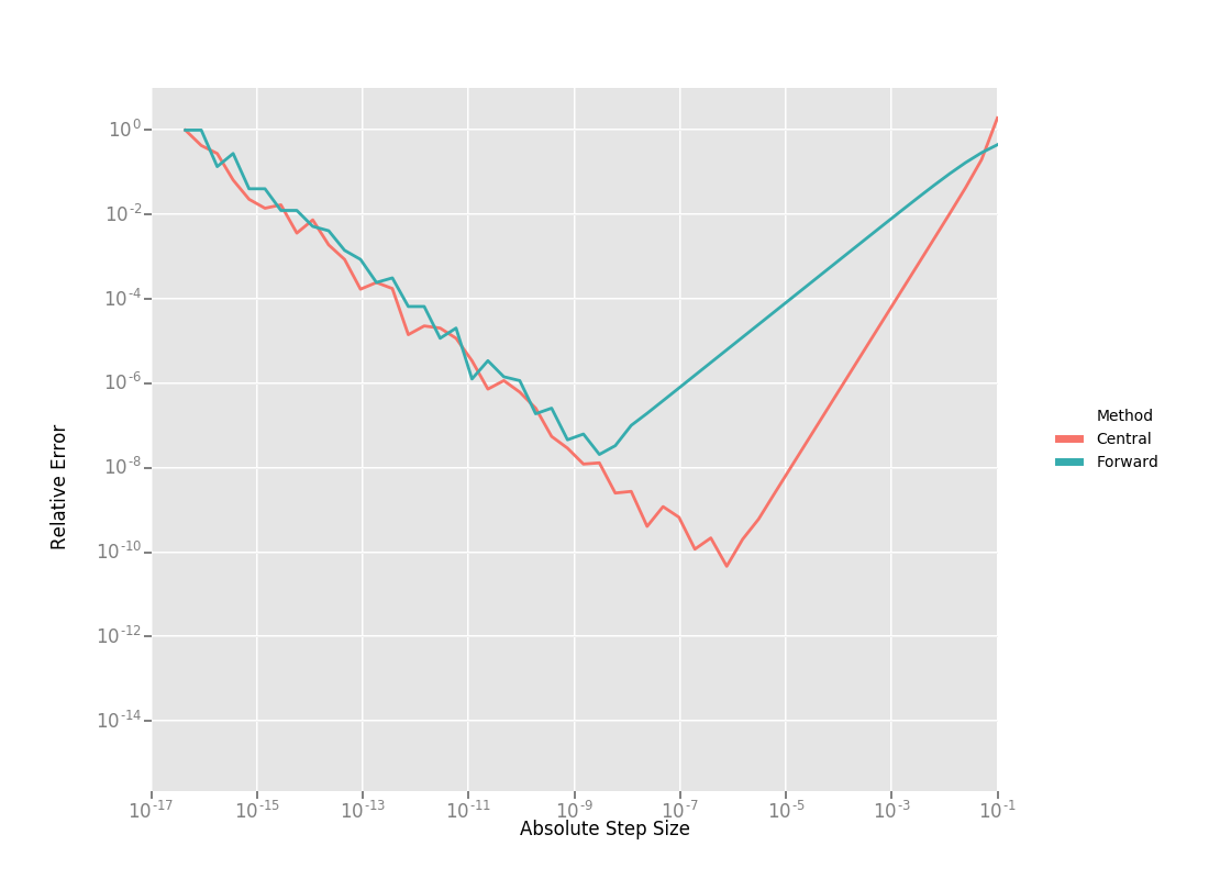
Reading the graph from right to left, a number of things stand out in the above graph:

1. The graph for both formulae have two distinct regions. At first, starting from a large value of \(h\) the error goes down as the effect of truncating the Taylor series dominates, but as the value of \(h\) continues to decrease, the error starts increasing again as roundoff error starts to dominate the computation. So we cannot just keep on reducing the value of \(h\) to get better estimates of \(Df\). The fact that we are using finite precision arithmetic becomes a limiting factor.

2. Forward Difference formula is not a great method for evaluating derivatives. Central Difference formula converges much more quickly to a more accurate estimate of the derivative with decreasing step size. So unless the evaluation of \(f(x)\) is so expensive that you absolutely cannot afford the extra evaluation required by central differences, do not use the Forward Difference formula.

3. Neither formula works well for a poorly chosen value of \(h\).

Ridders’ Method

So, can we get better estimates of \(Df\) without requiring such small values of \(h\) that we start hitting floating point roundoff errors?

One possible approach is to find a method whose error goes down faster than \(O(h^2)\). This can be done by applying Richardson Extrapolation to the problem of differentiation. This is also known as Ridders’ Method [Ridders].

Let us recall, the error in the central differences formula.

\[\begin{split}\begin{align} Df(x) & = \frac{f(x + h) - f(x - h)}{2h} + \frac{h^2}{3!} D^3f(x) + \frac{h^4}{5!} D^5f(x) + \cdots\\ & = \frac{f(x + h) - f(x - h)}{2h} + K_2 h^2 + K_4 h^4 + \cdots \end{align}\end{split}\]

The key thing to note here is that the terms \(K_2, K_4, ...\) are independent of \(h\) and only depend on \(x\).

Let us now define:

\[A(1, m) = \frac{f(x + h/2^{m-1}) - f(x - h/2^{m-1})}{2h/2^{m-1}}.\]

Then observe that

\[Df(x) = A(1,1) + K_2 h^2 + K_4 h^4 + \cdots\]

and

\[Df(x) = A(1, 2) + K_2 (h/2)^2 + K_4 (h/2)^4 + \cdots\]

Here we have halved the step size to obtain a second central differences estimate of \(Df(x)\). Combining these two estimates, we get:

\[Df(x) = \frac{4 A(1, 2) - A(1,1)}{4 - 1} + O(h^4)\]

which is an approximation of \(Df(x)\) with truncation error that goes down as \(O(h^4)\). But we do not have to stop here. We can iterate this process to obtain even more accurate estimates as follows:

\[\begin{split}A(n, m) = \begin{cases} \frac{\displaystyle f(x + h/2^{m-1}) - f(x - h/2^{m-1})}{\displaystyle 2h/2^{m-1}} & n = 1 \\ \frac{\displaystyle 4^{n-1} A(n - 1, m + 1) - A(n - 1, m)}{\displaystyle 4^{n-1} - 1} & n > 1 \end{cases}\end{split}\]

It is straightforward to show that the approximation error in \(A(n, 1)\) is \(O(h^{2n})\). To see how the above formula can be implemented in practice to compute \(A(n,1)\) it is helpful to structure the computation as the following tableau:

\[\begin{split}\begin{array}{ccccc} A(1,1) & A(1, 2) & A(1, 3) & A(1, 4) & \cdots\\ & A(2, 1) & A(2, 2) & A(2, 3) & \cdots\\ & & A(3, 1) & A(3, 2) & \cdots\\ & & & A(4, 1) & \cdots \\ & & & & \ddots \end{array}\end{split}\]

So, to compute \(A(n, 1)\) for increasing values of \(n\) we move from the left to the right, computing one column at a time. Assuming that the primary cost here is the evaluation of the function \(f(x)\), the cost of computing a new column of the above tableau is two function evaluations. Since the cost of evaluating \(A(1, n)\), requires evaluating the central difference formula for step size of \(2^{1-n}h\)

Applying this method to \(f(x) = \frac{e^x}{\sin x - x^2}\) starting with a fairly large step size \(h = 0.01\), we get:

\[\begin{split}\begin{array}{rrrrr} 141.678097131 &140.971663667 &140.796145400 &140.752333523 &140.741384778\\ &140.736185846 &140.737639311 &140.737729564 &140.737735196\\ & &140.737736209 &140.737735581 &140.737735571\\ & & &140.737735571 &140.737735571\\ & & & &140.737735571\\ \end{array}\end{split}\]

Compared to the correct value \(Df(1.0) = 140.73773557129658\), \(A(5, 1)\) has a relative error of \(10^{-13}\). For comparison, the relative error for the central difference formula with the same step size (\(0.01/2^4 = 0.000625\)) is \(10^{-5}\).

The above tableau is the basis of Ridders’ method for numeric differentiation. The full implementation is an adaptive scheme that tracks its own estimation error and stops automatically when the desired precision is reached. Of course it is more expensive than the forward and central difference formulae, but is also significantly more robust and accurate.

Using Ridder’s method instead of forward or central differences in Ceres is again a simple matter of changing a template argument to NumericDiffCostFunction as follows:

CostFunction* cost_function =
  new NumericDiffCostFunction<Rat43CostFunctor, RIDDERS, 1, 4>(
    new Rat43CostFunctor(x, y));

The following graph shows the relative error of the three methods as a function of the absolute step size. For Ridders’s method we assume that the step size for evaluating \(A(n,1)\) is \(2^{1-n}h\).

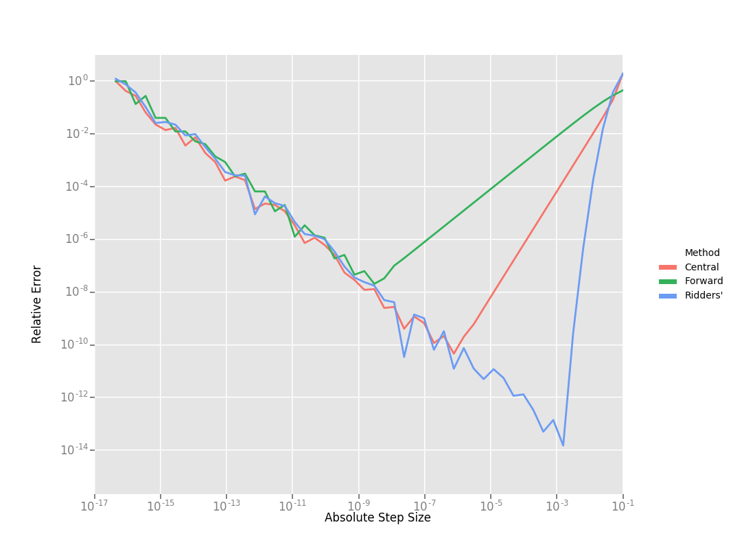
Using the 10 function evaluations that are needed to compute \(A(5,1)\) we are able to approximate \(Df(1.0)\) about a 1000 times better than the best central differences estimate. To put these numbers in perspective, machine epsilon for double precision arithmetic is \(\approx 2.22 \times 10^{-16}\).

Going back to Rat43, let us also look at the runtime cost of the various methods for computing numeric derivatives.

CostFunction	Time (ns)
Rat43Analytic	255
Rat43AnalyticOptimized	92
Rat43NumericDiffForward	262
Rat43NumericDiffCentral	517
Rat43NumericDiffRidders	3760

As expected, Central Differences is about twice as expensive as Forward Differences and the remarkable accuracy improvements of Ridders’ method cost an order of magnitude more runtime.

Recommendations

Numeric differentiation should be used when you cannot compute the derivatives either analytically or using automatic differentiation. This is usually the case when you are calling an external library or function whose analytic form you do not know or even if you do, you are not in a position to re-write it in a manner required to use Automatic Derivatives.

When using numeric differentiation, use at least Central Differences, and if execution time is not a concern or the objective function is such that determining a good static relative step size is hard, Ridders’ method is recommended.

Footnotes

[1]

Numerical Differentiation

[2]

[Press] Numerical Recipes, Section 5.7

[3]

In asymptotic error analysis, an error of \(O(h^k)\) means that the absolute-value of the error is at most some constant times \(h^k\) when \(h\) is close enough to \(0\).